Basic Theory
In statistical terms, we use the mixed-Poisson model for the observed count data, where the mixing distribution is a member of a parametric family (e.g., lognormal) that is indexed by a small number of parameters (typically 2 or 3). The observed count data is used to estimate these parameters, and the parameter estimates are used in turn to estimate the number of species and its standard error, and to assess the goodness-of-fit of the model. For a brief technical outline of this theory see Bunge and Chao (2002).
From an applied perspective, this model works as follows. Assume there are in fact a total of C classes or species in the population; C is the unknown quantity that we wish to estimate. Each species has a sampling intensity associated with it: this is the number of representatives (individual members) of the species that we expect to enter the sample given one unit of sampling effort. Note: if the sampling procedure is completely "transparent" relative to the population structure, then the sampling intensity will be proportional to the size of the species in the population. However, this is not typically the case: often the sampling procedure entails a series of intervening steps so that the sampling intensities do not exactly reflect the actual relative sizes of the species in the population (although they will typically follow the sizes monotonically: smaller species have lower intensities and and larger species have larger ones).
Unless we assume that all sampling intensities are equal, which is unrealistic and almost never fits real datasets, we must allow that the intensities differ from species to species. This variation can be rather extreme: in many cases there are a few very large intensities and a large number of very small intensities. We cannot estimate these C unknown numbers directly. However, if we assume that the C sampling intensities follow some parametric distribution (that is, that their histogram resembles the graph of some parametric probability density function), then instead of attempting to recover the C unknown sampling intensities we need only recover the parameters that determine the distribution. That is, we can describe the C intensities using only the 2 or 3 parameters of the distribution, no matter how many species there are. To put it another way, we will smooth the histogram of the intensities using some given parametric distribution. The parameters of the distribution are estimated from the observed count data using the method of maximum likelihood; ML estimation poses a non-trivial computational problem in this case, which is why we are developing specialized software.
We are usually not primarily interested in the underlying (sometimes called "latent") intensity distribution. However, the model also yields a smooth curve fitted to the plot of "frequencies of frequencies," i.e., the number of species observed once, twice, and so on. If we project this curve to the left, as the frequency (on the horizontal axis) declines to 0, we get an estimate of the number of species observed zero times, that is, the number of unobserved species. Adding this to the number of species observed in the data, we get an estimate of the total number of species in the population. The fit of a particular model can be assessed visually from the plot, and in addition we can apply the classical chi-square test to obtain a p-value for a quantitative goodness-of-fit rating. If we carry out the entire procedure for several different parametric models, we can then compare their performance and select the "best" -- although definition of the "best" is multi-dimensional (see below).
At the present stage of development, the above procedure poses the basic question: "Which parametric model should we use?" Unfortunately neither statistics nor applied science can answer this question at this point. There is no fundamental theory of "speciation" that gives rise to a particular model, and even if there was (or if one is established in the future), it is not clear whether its properties would survive the subsequent sampling steps: an ideal model would have to account for both the underlying structure of the population and the scientific processes required to obtain the count data. Furthermore, even if a given model is found to fit in a certain applied situation, there is no reason to suppose that it will fit in a different situation or even in a future study of the same population. Given these considerations, our approach must be primarily phenomenological: what fits the data?
An example
Here is a short, simplified example based on a simulated dataset (which was adapted from a real dataset). The count data is as follows.
| frequency | frequency of frequencies |
|---|---|
| 1 | 21 |
| 2 | 8 |
| 3 | 5 |
| 4 | 2 |
| 5 | 4 |
| 7 | 1 |
| 8 | 2 |
| 12 | 1 |
| 14 | 2 |
| 15 | 1 |
| 17 | 1 |
| 24 | 1 |
| 27 | 1 |
In other words, there were 21 species observed only once (21 "singletons"); 8 observed twice, and so on. This structure, with a "spike" left-ward toward 1, i.e., a relatively high number of singletons, and a long right-hand "tail", i.e., some very abundant species, is typical. One of the main objectives of statistics in this area is to find parametric models that will fit complete datasets of this type; however, most existing models can accommodate either the left or the right side of the frequency distribution but not both. Based on the intuition that the left side (the lower frequencies) contain more information about the zero frequency (the number of unobserved species) than the right side, we fit the largest amount of the data (the highest possible right truncation point) that fits the data, and then add in the more abundant species having observed counts larger than the right truncation point.
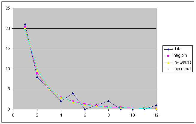
In this example one reasonable right truncation point is t = 12. (The choice of the right truncation point in parametric models is part of the general problem of model selection, which is multi-dimensional.) The result of fitting the negative binomial, the inverse Gaussian, and the lognormal to the frequency counts up to 12 is shown in the following graph.

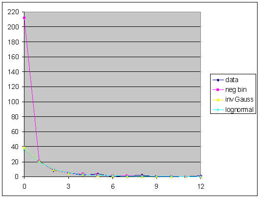
All of these models fit the data well (at this right truncation point), both impressionistically and by standard goodness-of-fit statistics. However, they do not give the same answer. If we project the curves upward to the left, we obtain the following plot.

The negative binomial model projects 212 unseen species, for a total estimate of 262 species, while the inverse Gaussian and the lognormal agree in projecting 38 and 36 (respectively) for total estimates of 88 and 86 (resp.). The divergence between the models is not as great as it might first appear, however, because the standard error for the negative binomial estimate is 611 (rendering the result almost useless), while the other two SE's are 20 and 25 (resp.). Thus the three models actually do not disagree, although the latter two are clearly preferable.
This example is mainly intended to illustrate the overall strategy and does not present the complexity that is usually encountered in real-world data analysis (we have even hidden some of the complications with this example). The actual output of the software.
