Introduction
In this project, we created a one-way communication system using a Raspberry Pi, a microphone, and a speaker. The speaker, acting as the transmitter in the system, was able to communicate arbitrary, fixed-length bit string frames to the Raspberry Pi by playing a series of tones, which the microphone recorded and the Pi processed to recover the bits. Bits were encoded using multiple frequency shift keying (MFSK), which assigns different tone frequencies to different combinations of bits, allowing for multiple bits to be sent in each transmitted symbol. By implementing a cyclic redundancy check, we were able to create a system that was fairly robust to noise and echoes; given the constraints of the frequency band that we were working with (about 350 Hz to 750 Hz), we did not expect to correctly receive every transmission, but we were able to at least detect whether a transmission was received without error.
Design & Testing
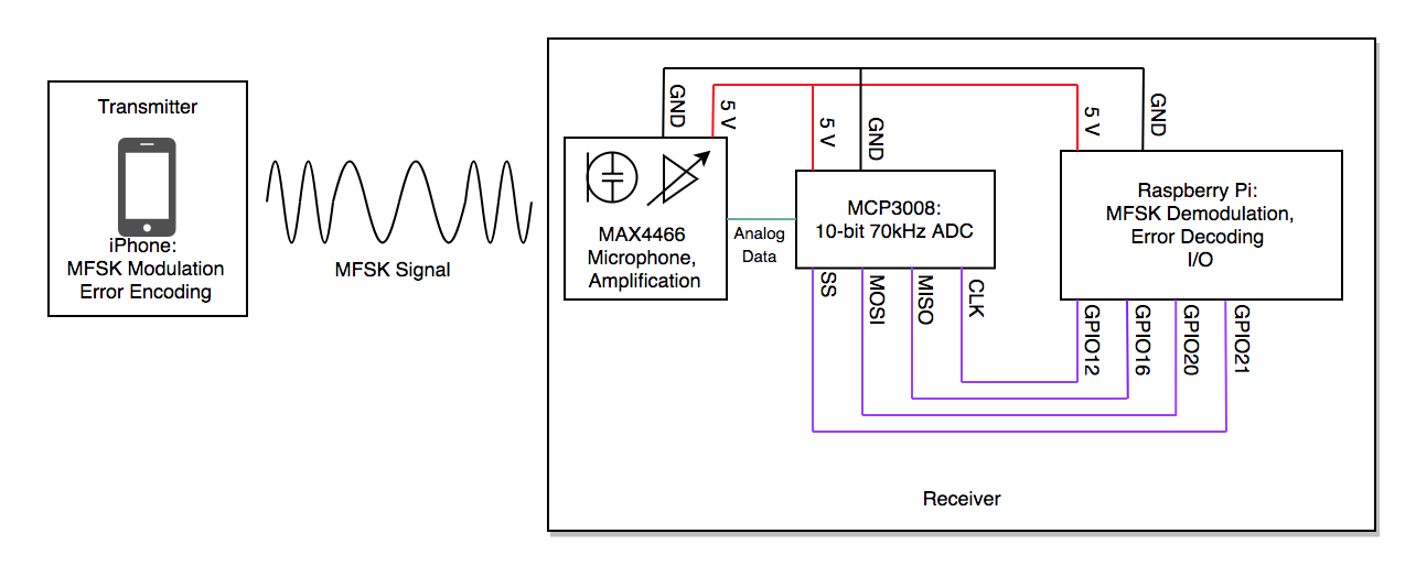
Our system uses software on the Raspberry Pi to demodulate received signals to extract the original information transmitted by an laptop transmitter. Demodulation is done primarily in software, with analog-to-digital conversion done in hardware. On the transmitter size, an laptop runs an application to modulate a series of bits into an MFSK signal. Figure 1 shows an overview of our system.
Hardware Design
Our project consisted of two hardware devices: a Raspberry Pi controlled receiver and a laptop controlled transmitter. Our Pi receiver consisted of a Raspberry Pi with the following peripherals: a PiTFT touchscreen with GPIO buttons, an MCP3008 10 bit analog-to-digital converter (ADC), and a MAX4486 electret microphone with adjustable gain. We used no peripherals for the laptop transmitter, opting for the built-in speakers.
Table 1 shows the peripheral inputs to our system. The output of the MAX4486 is connected to channel 0 of the MCP3008. This communicates the received analog signal for analog-to-digital conversion.
| Purpose | Raspberry Pi Pin |
|---|---|
| ADC CLK | GPIO12 |
| MOSI | GPIO20 |
| SS | GPIO21 |
| Quit Button | GPIO27 |
| Mute Button | GPIO17 |
We originally intended to use an ADS1115 12-bit ADC, for both its adjustable gain and its precise resolution. However, after ordering the part, we realized that the maximum possible data rate was 860 samples per second, which (by the Nyquist sampling theorem) would have constrained us to frequencies below 430 Hz and crippled our data rate. We found the MCP3008, which has a sampling rate of more than 75,000 samples per second at our supply voltage, which worked much better for our purposes.
When debugging the microphone circuit, the oscilloscope was our tool of choice. The microphone had a tunable gain, adjustable using a potentiometer, and we determined the maximum gain point by playing a tone into the microphone and adjusting the pot until the amplitude on the oscilloscope was maximized. When we were trying to detect ultrasonic frequencies, we were able to see on the oscilloscope that the amplitude was too low for our ADC to give us accurate resolution, allowing us to move on with the project without sinking additional hours into determining why our fast Fourier transform was not detecting any peaks. We also used to oscilloscope to verify the correctness of the encoder output, by using the measure function to determine the received frequency of the sinusoid.
Software Design
We needed a way to encode bits into a sound such that it would be feasible for the Pi to recover the original bits from the received sound. Each bit, or potentially chunk of bits, is assigned a time slot in which to be transmitted. A naive approach to encode the bits in each time slot might be to play a loud sound for a one, and send silence for a zero. This approach is called amplitude modulation, and for our purposes, it would not work: the microphone received a much quieter copy of the signal, and any loud sound in the lab during a “silence” period would result in a decoding error. We knew that some sort of frequency modulation would be required; while the microphone might mangle the received signal amplitude, because it’s well modeled as an linear time-invariant (LTI) system, it would not shift the transmitted frequencies.
Frequency shift keying (FSK) is one of the simplest frequency modulation schemes, and it was a perfect match for our setup: we didn’t need something as complicated as OFDM (orthogonal frequency division multiple access), since we were not worried about channel sharing, FSK is highly noise-tolerant (needed because of the quality of our microphone), and FSK can be decoded with reasonable computational complexity (needed because this is a real-time application). FSK encodes bits by sending a sinusoid in each time slot, and varying the frequency of the sinusoid depending on the data to be sent. For standard FSK, there are only two frequencies, one for sending a “1” bit and one for sending a “0.” MFSK (multiple FSK) sends more than two frequencies so as to encode more than one bit in a single tone; we settled on using 2FSK (four frequencies in total), allowing us to send two bits with each tone. We tested 4FSK, but the narrowness of our frequency band and the noisiness of our channel prevented us from distinguishing neighboring tones.
Encoder
The encoder, as is often the case in communications systems, was much less complex than the decoder. Each block of two bits was mapped to a frequency, and a sinusoid was played with that frequency for the duration of the time slot. Table 2 shows the mappings from bits to frequencies. The maximum symbol rate we could sustain through the channel was 4 symbols per second, so each encoded sinusoid was played for 250 ms.
| Bits | Frequency |
|---|---|
| 00 | 400 |
| 01 | 500 |
| 10 | 600 |
| 11 | 750 |
Each transmission from the encoder was made up of a start-of-transmission signal, a prefix frame, and a data frame. The start-of-transmission signal was included to make it possible for the receiver to detect the start of a transmission from the transmitter. A special two-tone chord was played with frequencies 350 Hz and 450 Hz for three time slots, allowing the decoder to look for a spike in power at those frequencies.
The prefix frame was constructed of four symbols, each the encoding of the bits 00, 01, 10, and 11, respectively. Sending this known sequence of bits at the beginning served two purposes. For one, it protected against the pathological “all zeros” case, which would otherwise be impossible for the decoder to determine as correctly transmitted; when the signal was sent from too far away, the start-of-transmission was often properly detected, but the rest of the transmission would only have one frequency detected, and the signal would appear to be only zeros. It also exposed the decoder to each of the possible transmitted symbols, making it possible to create decision boundaries on the demodulated signal.
Finally, the data frame was composed by concatenating each of the 250 ms sinusoids, with the MSB of the transmission being transmitted first.
Decoder
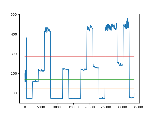
The decoder provided much of the signal processing involved in this project, as it had to probabilistically guess the bits sent by the transmitter by means of Bayesian inference. To simplify our design, we modeled our channel as an additive white gaussian noise (AWGN) channel, allowing for our maximum likelihood decision regions to be the governed by the minimum distance rule. An example of the minimum distance rule applied in our project is shown in figure 2. Another challenge the decoder faced was detecting the start of a real transmission; this is discussed in the section on synchronization.
The Pi sampled from the microphone at 7500 Hz, allowing for a maximum frequency component of 3750 Hz in the transmitted signal. Due to the gain of the microphone at different frequencies (and the unpleasantness of playing high pitched sounds) we kept our transmitted frequencies below 800 Hz. Given our 10-bit ADC and a 3.3 V supply voltage, the ADC grouped voltages into roughly 3 mV bins, with a total of 1024 bins.
Because of the real-time nature of our application—in particular, the sensitive timing of sampling from the microphone—we needed to make sure that our decoder process was not interrupted by other processes running on the processor. To accomplish this, we added a flag in our /boot/cmdline.txt to instruct the Pi not use one of the four cores, and we used the Linux taskset utility when running the decoder script to force the decoder to run on the isolated core. We verified using the Linux perf utility that the number of context switches was dramatically reduced by doing this.
In order to properly guess the original bits, our receiver needed to demodulate the received signal. Demodulation started after analog-to-digital conversion, allowing for all signal processing to be performed in software.
First, we needed to separate our encoded information from the carrier signal. To do this, the decoder differentiated the received signal. Next, we used a low pass filter to isolate the digital data. At this point, we sampled the filtered signal at the midpoint of each data slot, and used the minimum distance rule to determine the original bits from the filtered signal, as described in the section on synchronization.
We wrote a Python script that simulated an encoded signal with AWGN, and passed that to the decoder. This allowed us to rapidly iterate on our decoder design without being concerned with waiting for actual transmissions and artifacts of the microphone recording. From our simulation, we obtained a rough estimate of what symbol rate we could achieve, and what levels of noise we could handle, which provided a good starting point when modifying our decoder to work on actual received signals.
Synchronization
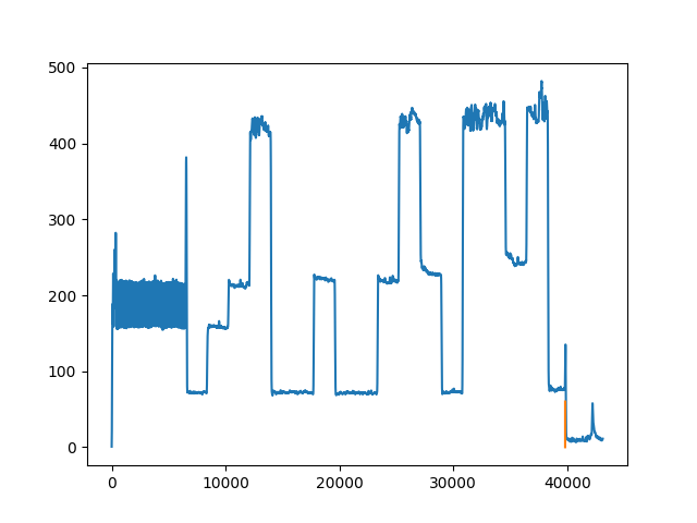
Our receiver continually listened for the start of a transmission, demarcated by the start chord described in the section on the encoder. The Pi recorded samples from the microphone for 250 ms, then searched that time slot for the start chord while recording the next time slot. The start signal was detected by doing a fast Fourier transform (FFT) on the samples, and comparing the magnitudes of the frequency components at the two frequencies of interest (350 Hz and 450 Hz) to the magnitudes of nearby frequencies. A spike in the magnitudes of both frequencies by a chosen threshold compared to the average magnitude of the frequencies around them was determined to be the start of a transmission, at which point the receiver would record for the duration of transmission. Start of transmission detection is shown in Figure 3.
The exact threshold to use for start detection was determined by trial and error. We wrote a script that sampled from the microphone continuously and plotted the FFT output every second. From these plots, we were able to see how much of a spike was being detected at the frequencies of interest, and how large of spikes were to be expected due to noise. Because of these tests, we realized that we should send two separate tones for the start signal, so that random noise fluctuation did not accidentally trigger recording.
Once the transmitted signal had been recorded, the position of the prefix frame needed to be determined. To do this, we scanned the demodulated signal backwards from the end of the recording, and looked for a spike in the signal from one block of samples to the next; this was possible because the recording, by design, always contained a small amount of silence from after the tone was done playing. We looked for a spike in a block of samples instead of looking on a sample-by-sample basis to prevent small perturbations due to noise from triggering our decoding at the incorrect position. Once the spike was detected, because we were transmitting a fixed frame size, we could back up enough samples to reach the beginning of the prefix frame. In practice, this start of prefix detection worked fairly well, but could be affected by the presence of too much ambient noise in the lab.
Our original technique to detect the start of the prefix frame was to scan from the beginning of the recording and look for a drop in the filtered signal. This drop was dependable using the set of speakers that we were primarily testing with, and can be seen in Figure 3. However, after trying this with different speakers, we found that some speakers had a drop from the start tone to the first symbol of the prefix, while others actually had a rise. This was due to the different gain of the speakers at different frequencies. After switching to the new start detection algorithm, we were able to get transmission working with other devices.
After the decoder filtered the signal, it used the known structure of the prefix frame and detected start of the prefix frame to determine decision regions for the filtered signal. Each symbol was relatively flat over the duration of its time slot; because the prefix frame was constructed to increase the frequency of the encoded signal monotonically, the prefix of the filtered signal looked like a staircase. The decision regions were chosen using the minimum distance rule, i.e., by averaging the filtered signal over each of the four prefix frames, and matching future samples to the nearest average.
Demo
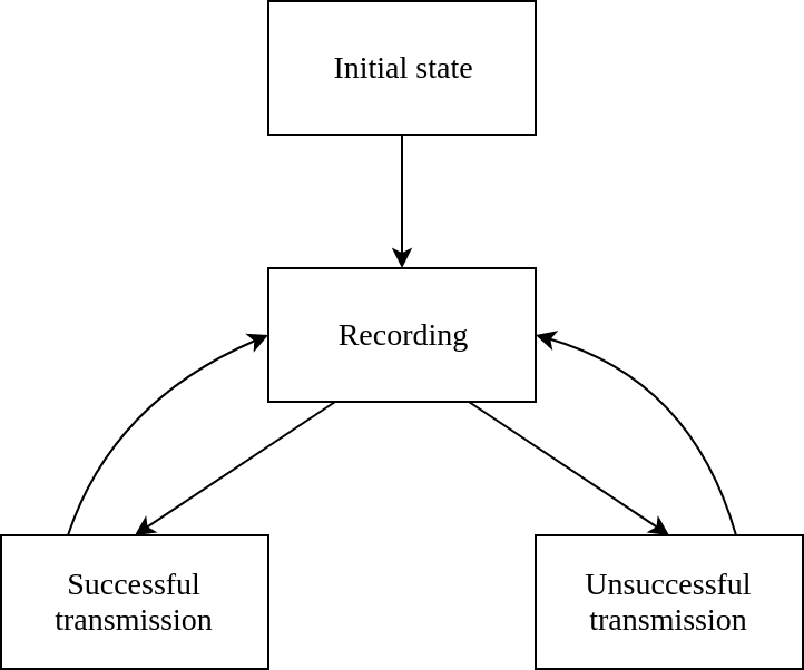
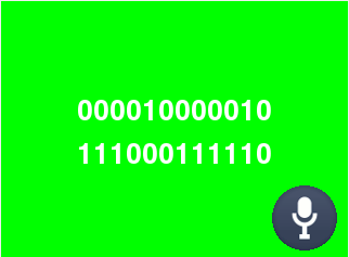
To demonstrate our communication system, we wrote an embedded application that ran on the Raspberry Pi and the PiTFT that listened for transmissions and displayed the transmission payload when properly detected. The application had four states:
- An initial state, in which no transmission has been detected yet, and the start of a transmission is being waited for
- A recording state, in which a transmission is being buffered for processing
- A successful transmission state, which displays the received bits
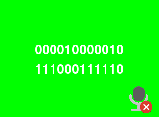
- An unsuccessful transmission state, which displays an error message indicating that the transmission was unsuccessful
Figure 4 shows a finite state machine diagram for the demo. The application was listening for the start of a transmission in every state except for “recording.” In each of those three states, button 17 on the PiTFT could be pressed to mute the microphone, which would stop the application from listening for a start signal until the microphone was unmuted.
Button 27 on the PiTFT could be used in any of the “listening” states (i.e. all of the states except for recording) to quit the application. Screenshots of the PiTFT screen in each of the different states are shown in Figure 5.


Results
We originally wanted to work in ultrasonic frequency bands but due to small gain in frequencies above roughly 7kHz, the MAX4486’s amplifier gain was lower than necessary in order of signals to be recorded properly; in these low gain regions, our decoder would decode an empty bitstream. However, in the frequency bands specified in the Design and Testing section, our decoder was able to perfectly decode information about 70% of the time when transmitted at an appropriate distance. The distance in which bits could be decoded properly varies with the power (volume) at which the transmitter can send signals. For a Lenovo IdeaPad, this distance was a few centimeters.
Unfortunately, we were not able to transmit using an iPhone as planned as the volume at which the iPhone played sound was too low for our receiver to decode, leading to high bit error rates.
Conclusion
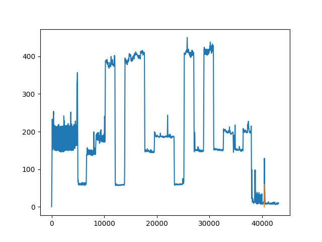
We were able to design and implement our communication system with reasonable success. Most packets were decoded properly, due to the nature of failure modes, packets with a single bit error are thrown out entirely, since bit errors are primarily caused by improper triggering by unanticipated local spikes in signal power. Failure to the detect the start of a signal effectively means all of your received data is unreliable, which is why we chose to throw out these packets. An example of an improper trigger is shown in Figure 6.
While developing this project. We primarily learned about the difficulty and importance of system synchronization and its necessity in real-time systems. Synchronization was heavily dependent on specific timing constraints, which made it susceptible to critical errors which can reasonably result in system failure. We were able to time the system very precisely with the PreemptRT kernel patch, but this was unfortunately not enough to defend against the unpredictable power spikes.
Future Work
As the original goal of this project was to communicate using ultrasonic frequencies, future work on this project would primarily be focused on updating our project to handle higher frequency bands. This can be achieved by upgrading hardware components used (primarily purchasing a more sensitive microphone and possibly constructing a preamplifier circuit) and with small modifications to our software at the encoder and decoder.
In addition, we would like to fix the issue of power spikes causing improper detection at the decoder. We believe that additional filtering during demodulation will help solve this problem. To improve robustness, we would like to improve our CRC code to fix bit-errors rather than simply detecting them.
Finally, we would work to get transmission working with a mobile phone. Because the encoder is a web application, it can be run on any device with a web browser. We had some success with using an iPhone as the transmitter, but the iPhone sound card seemed to try to "smooth" the transitions between the frequencies, which made the decoding much harder. It also introduced issues with volume control that we did not have time to address; for example, when playing the start chord, the chord would start at full volume and then quickly become quieter without us adjusting the volume.
Work Distribution
Joao Pedro: Hardware and software design and implementation. Report writing: overview, hardware design, decoding, synchronization, results, conclusion.
Angus: Hardware and software design and implementation. Report writing: software design, testing, synchronization.
Project Parts
| Part Name | Price (USD) | Link |
|---|---|---|
| Raspberry Pi 3 | 35 | https://www.raspberrypi.org/products/raspberry-pi-3-model-b/ |
| MCP3008 | 3.75 | https://www.adafruit.com/product/856 |
| MAX4466 | 6.95 | https://www.adafruit.com/product/1063 |