Vibration Diagnostic Tool for Machine Health

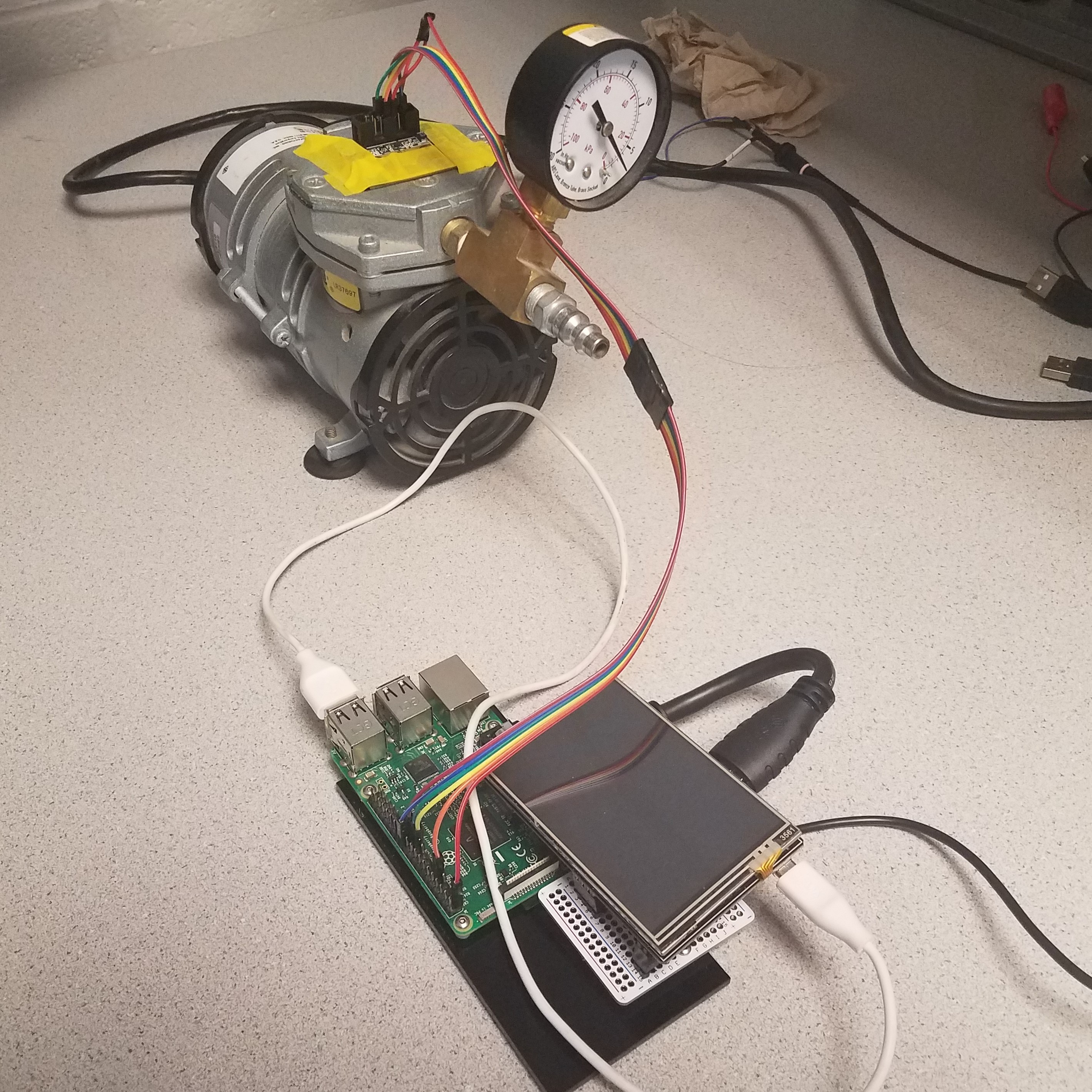
Final Machine Health Diagnostic Tool

The main tasks the system would have to perform were to collect data from an accelerometer, parse the data into chunks, perform an FFT on the data, and update a small display showing the FFT graph in real-time. For the accelerometer communication and data collection, we used the raspberry pi’s SPI0 module with the BCM2835 C GPIO library.

The data collection was done using C code in order to attain fast collection speed. The C code then transferred the data to a FIFO object in the pi which was read by a python script. The python script collects the data in chunks of 2048 data points and then performs an FFT on the collected data points. Both the array parsing and the FFT calculations were handled using the numpy library module. Once the FFT is calculated, the python script uses the matplotlib library module for the plotting aspect of the project. A fullscreen interactive plot is generated by the script on the 3.5” HDMI display which updates whenever new FFT data is available. Both the C and python scripts are in a bash script which runs at boot up to the desktop environment, so no user interaction is needed to start the system.

Data Processing Flowchart

For the physical aspect of the system, the raspberry pi and the display were secured using screws to a piece of laser cut acrylic, and the accelerometer board was attached via ribbon cable and for the purposes of the demo, was secured to the air pump using electrical tape. Ideally, the accelerometer should be secured using screws or a similar fastening method to the machine being monitored.

Machines such as turbines, pumps and compressors degrade over time and many of the faults can be diagnosed by vibration analysis techniques such as the Fast Fourier Transform (FFT). This project aimed to create a raspberry pi based portable system to diagnose machine health issues using mechanical vibration analysis.

Hardware - The Accelerometer and Pi

For the accelerometer, we selected the Kionix KX023 3 axis accelerometer. The accelerometer “officially” supports data output rates up to 1600 Hz, and can communicate using SPI up to 10 MHz and I2C up to 3.4 MHz. Although the rates officially supported only go up to 1600 Hz, by writing a value of 0x0F to the ODCNTL register, you can put the accelerometer into a debug mode where it collects data at 25.6 kHz. This mode isn’t supported by the company, and was only known due to a group member's familiarity with Kionix products. We used this debug mode to achieve the fastest possible sampling rate to be able to measure the largest spectrum of frequencies. By nyquists sampling theorem:

Fsamp = 2Fmax

We can measure signals up to 12.8 kHz without aliasing. The accelerometer also has many integrated features, such as built in low pass filter, and many available interrupt functionalities. For our project, we only utilized the data ready interrupts for debugging and verification; these interrupts generate a pulse whenever a new data point is given by the accelerometer. We used these interrupts to ensure that the data is being generated at the intended rate, this is important because if a data read takes too long and isn’t done before the next point is generated, the data rate will drop. This was very important for us to be sure of because of the unofficial mode we were running the accelerometer in. The KX023 can’t run at any data rate between 1.6 kHz and 25.6 kHz, so if the data rate dropped from 25.6 kHz it would drop down to 1.6 kHz.

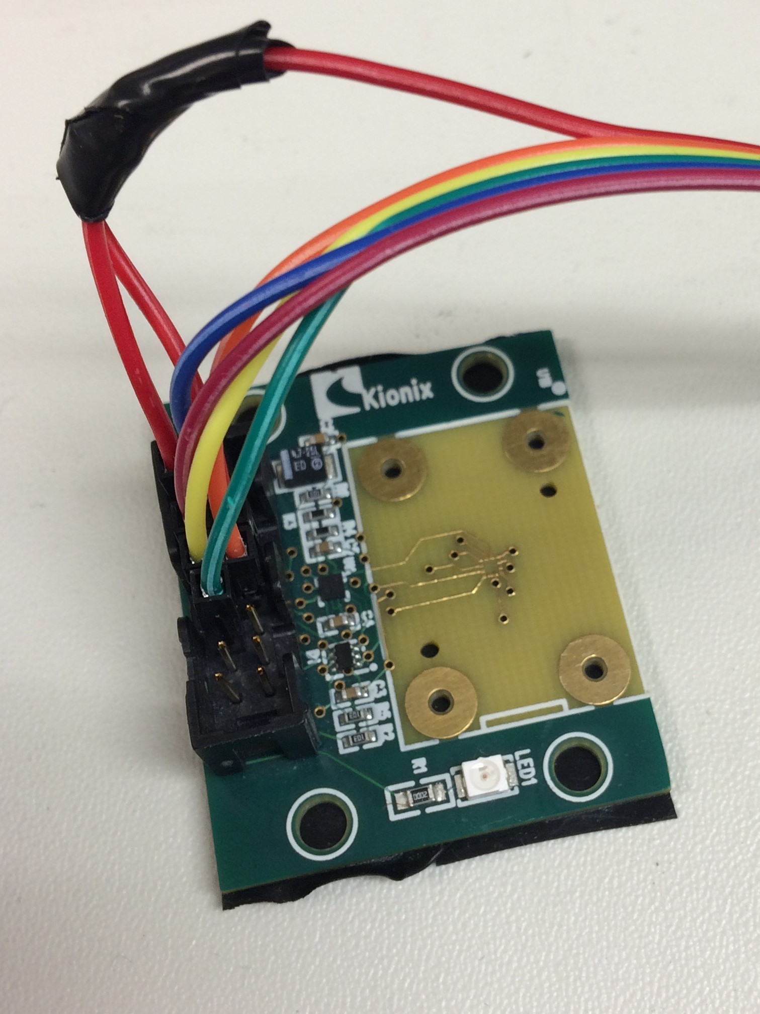
KX023 Accelerometer

We used 4-wire SPI protocol to communicate with the accelerometer. We used the SPI channel 0 SCLK, MOSI, MISO and CE lines to connect to the SCL, SDA, SDO and CS lines on the accelerometer boards respectively. We also probed the INT1 line for the data rate debugging mentioned earlier, but it is not part of the final system. The VDD and GND lines on the accelerometer were connected to the 3v3 and ground lines of the raspberry pi respectively.

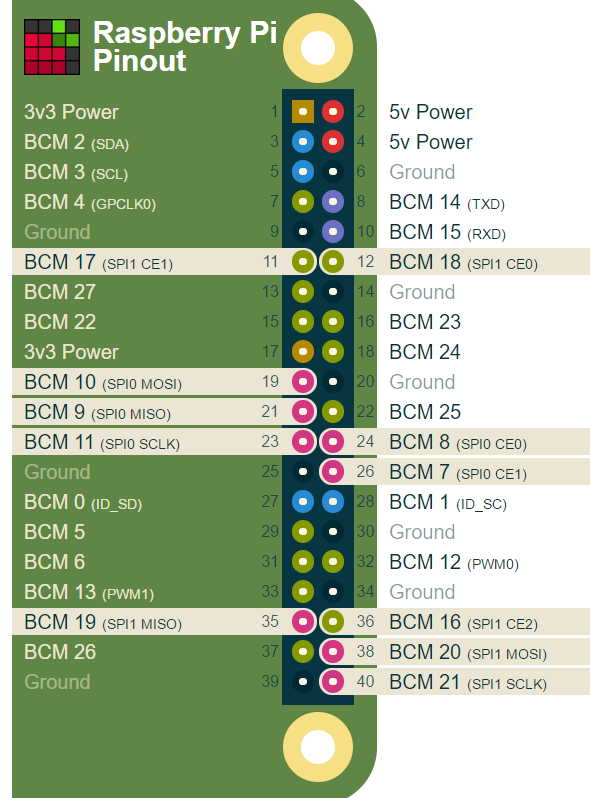
WiringPi Pinout for SPI

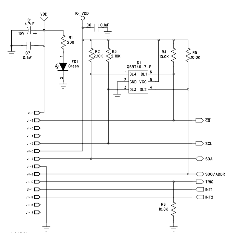
Board Diagram from KX023 Datasheet showing Breakout Pin to SPI Pin Mappings

For the display, we used the kedei 3.5” HDMI screen. This screen was chosen because unlike the TFT supplied in lab, the HDMI screen does not use the SPI0 channel to communicate and send data to and from the Pi, so that channel was free to use for the accelerometer. Despite not using the SPI0 pins, the screen is designed to secure onto the top of the Pi using the headers for the SPI0 pins. For that reason, our physical model had to secure the screen in a different way covered in the physical model section.

Software - Overview

The software side of the project consisted of two main parts, a C program that handled data collection from the accelerometer, and a python script that parsed the data into arrays, performed an FFT on it, and updated a live plot of the data. The go-between method for the two scripts was FIFO file object.

Software - SPI Setup and Data Gathering

In order to make sure as little data was missed as possible, and that no data reads would be delayed and potentially drop the data rate, a standalone C script was written to handle communication and data collection with the KX023. The script was designed to run as fast as possible which is why it was written in C code rather than python. The scripts only functionality was to collect data via SPI and write it to the FIFO.

For SPI communication, we used the BCM 2835 C library. This library was used by a group member in a similar past project for SPI data collection, so familiarity with the library was a major factor in the choice. When using SPI, it is important to understand the simultaneous aspect of it. When the Pi is performing a write for a byte, it is simultaneously reading a byte as well (usually garbage). Inversely, when the Pi wants to read a byte, it needs to write one simultaneously. Many libraries provide spi write and read functions, which take care of the garbage being written or read, but in the experience of this project, these functions were inconsistent. As a result all writes and reads were handled by the transfer function rather than the read or write ones. The transfer SPI function takes as an input a buffer of data to write across the line and a buffer of data to read data into. This nuance in the SPI communication is important because of the data buffers that need to be sized accordingly. In accordance with the KX023’s communication protocol, in order to write data to a register (to for example setup the accelerometer), first the register address must be written with a ‘0’ in the MSB, then the data is written. To perform a write a 2 byte buffer variable of data (register address and data) is the write input to the transfer function, and an empty 2 byte buffer is the read input to the function. The empty two byte buffer receives meaningless data and is thrown out or over written. In order to read from a register, the register address must be written to the accelerometer with a ‘1’ in the MSB, then the accelerometer will send the data in the requested register. So for a two byte read, a 3 byte buffer variable must be in the transfer function read and write inputs. For the write buffer, the first byte is the register address with a ‘1’ in the MSB, and the 2nd and 3rd bytes are zero. For the read buffer, all bytes are zero, but the 2nd and 3rd bytes will contain the read data after the transfer.

The C program begins by initializing the SPI communication with the proper settings which were pretty common for SPI and were as follows:

• The chip select pin is active low
• SPI clock to 6.8 MHz (set by a divider, this is the highest it could go)
• SPI mode 3
• Chip select pin is CE0

The program then writes the values to the accelerometer registers to set up the following settings:

• 2g range
• 16-bit data resolution
• Data Ready interrupts on the INT1 pin
• 25.6 kHz data rate
• Start data collection

The program then enters a while loop were it reads the Z-axis data and writes it to the FIFO. The data collected for the Z-axis consists of two bytes, the high eight bits and the low eight bits. After the data is received, the two unsigned bytes are combined into an unsigned 16 bit integer before being written to the FIFO using the fprintf function. It is important to note that the data point is written to the FIFO as a string.

Software - Data Processing and Visualization

The python script on the other side of the FIFO was responsible for reading the data from the C script, parsing it into arrays for the FFT function to process, and then plotting the FFT results on the HDMI display. The python modules we needed to install were numpy for array management and the FFT function, and matplotlib for the plotting. For the FFT, we used the rFFT function, which is the FFT algorithm optimized for when the input data is all real and not complex.

The program begins by initializing the FFT parameters based on the sampling time of the accelerometer and the number of points in each array of data. The FFT algorithm used by numpy works most efficient for array whose size is a power of 2, we chose 2048 somewhat arbitrarily. The number of points is definitely a tuning parameter that can be messed with to affect the performance of the program. For the X-axis of the FFT plot, the points are generated at the beginning of the program by the rFFTfreq function. This function generates the “bins” corresponding to the FFT values using the number of points in the data and the data sampling rate. For the initial plot, an FFT of all zeros is plotted against the x-axis points. The parameter for the plot are then setup using the appropriate matplotlib functionalities:

• Interactive plotting (enables updating of the data in the plot without redrawing the plot)
• X-axis from 0-800 Hz (mechanical vibrations won’t go above that very often)
• Fullscreen plot

The python function then enters a loop where it reads from the FIFO and converts each data point from a string back to an unsigned int. The unsigned int is then converted to a signed int using a 2’s complement conversion function and then converted to a float value of g’s using the counts to g’s conversion factor:

0.00006104 = 2g resolution/ 32767 counts in decimal

The float calculation was truncated at four decimal places based on the resolution of the readings. Before the rFFT was implemented, values being read through the C program and processed through the python program were confirmed by reading out all three axis of data and making sure the value read about -1g when the positive axis of the board was facing up. The function then concatenates the value with the collection array until it has 2048 values. Once the size of the array hits 2048, the array is passed through the rFFT function, then the plot Ydata property is updated with the output of the rFFT function and the plot is updated.

Software - Linux System Configuration

In addition to the C and python code, there were some adjustments to our raspberry pi’s linux system to get the system to operate as intended. In order to increase performance, we wanted to isolate the two different scripts on different cores of the raspberry pi. We did not want the two processes pre-empting each other. When we ran the scripts, we used the taskset command to run the python script on core 3 and the C script on core 2.

We also needed the scripts to run at startup, which proved to be more difficult than running a simple servo control script from a previous lab. The complication stemmed from the fact that since the python script involved plots, a display environment was needed. The desktop environment needed to be booted up before the python script ran, otherwise it would throw an error and exit. We configured our Pi to autologin to the desktop environment at startup. In a previous lab we ran scripts at startup by adding the linux command to run the script into the rc.local bash script. The problem with this method is that rc.local runs directly after booting of the Pi, and before the desktop is booted. We tried not configuring the Pi to boot to the desktop, and instead putting startx and a sleep command in our bash script before running the script, but then we ran into a login error on the desktop. We also had an issue where we had left an incorrect command in another bash script while trying to edit another script to work. Eventually after much research we discovered a script we could edit to run a bash script when the LXDE desktop environment is booted. The script was found in the following file, within the LXDE directory:

/.~config/lxsession/LXDE/autostart

We created a bash script that ran the python script and then the c script and added the following line to the autostart file. This allowed us to link the bash script to the booting of the LXDE desktop environment:

@bash /home/pi/FinalProject/Accelerometer/startup.sh

Physical Design
Our physical design of our system was a little convoluted due to the HDMI screens header stands taking up the SPI pins, and therefore not allowing us to simply place the screen on top of the pi. We decided to secure both the pi and the screen to a piece of laser cut acrylic with screws. For the screen, we soldered headers to a protoboard to plug in the display, then secured the proto board with screws. The accelerometer board was attached to the pi using ribbon cable secured with electrical tape. As mentioned earlier, the accelerometer board was secured to a compressor using electrical tape for the sake of them demo, but ideally it should be secured using screws.

SPI Woes

Initially, we wanted to use the TFT supplied by lab for the display, however that used the SPI0 channel. This meant we needed to use the SPI1 channel for communication with the accelerometer. The SPI1 channel on previous Raspberry Pi models wasn’t broken out to the header pins, and as a result many of the Pi GPIO C libraries do not have support for more than one SPI channel. The pigpio C library does have support for the SPI1 channel, so first attempts at development of the C code was attempted using the pigpio library. This library proved to present many odd problems during development. The SPI communication was not working using known SPI working code with only the channel changed. Our code to communicate with the accelerometer was not collecting data which we confirmed with the oscilloscope (no lines were transmitting). The only time we were able to get the lines to show transmission was when we transmitted a very large amount of data, and still what was read back was garbage. Due to SPI1 being relatively new as an available periphery, there is surprisingly little documentation on these issues at time of writing. When we realized the alternative option of using an HDMI display instead of a SPI one, freeing up SPI0, we decided our time was better spent doing that and moving on.

Verifying SPI

To verify we were not missing data we probed the MOSI line of the Pi to make sure Verification of accelerometer data was done by converting the raw data in the C program and printing it to the console. We checked each axis by placing the positive side upwards and verifying the output value was equal to the acceleration due to gravity. We then moved the accelerometer to verify the values changed in the correct direction when a positive or negatvie acceleration was applied. To verify that the Pi and accelerometer were communicating at the desired speed and that no data points were being lost, we probed the Pi's MOSI pin. An example output of the scope can be seen in the figure below.

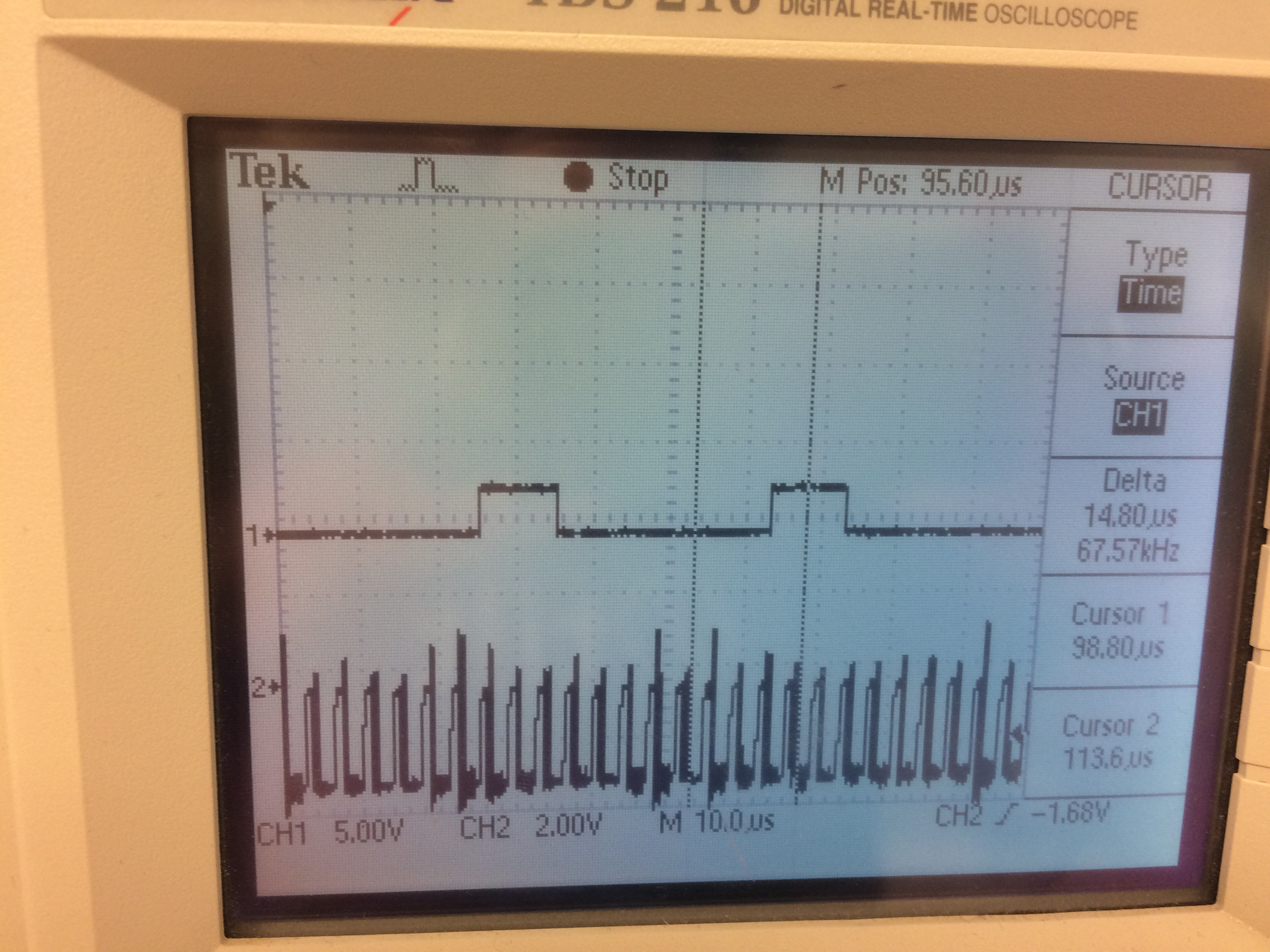
Scope Output of Pi's MOSI Pin

Testing the System

Testing of the integrated system was done using several machines that exhibited sizeable vibrations when running. Preliminary testing was done on a large drill press as well as a sander. The accelerometer was mounted using tape and the system collected data as the machines ran. Due to the size of these machines compared to their actual moving parts, the amplitude of the vibrations was fairly small. However, even at these levels the returned plots resembled what one would expect. These machines were running at a few thousand rpm and the plot as expected hovered between 20 and 60 Hz. Testing and the final demo were also done on a small ari compressor as it was more portable. The amplitude of vibrations were much larger for this machine and therefore the resulting plot was cleaner. We were not able to test on any machines that had problems such as a loose parts or bad bearings that would cause abnormal vibrations, however it would be highly beneficial to asses the feasibility of using this tool for machine health by testing on a perfectly working machine then breaking the machine in some manner and testing on it again.

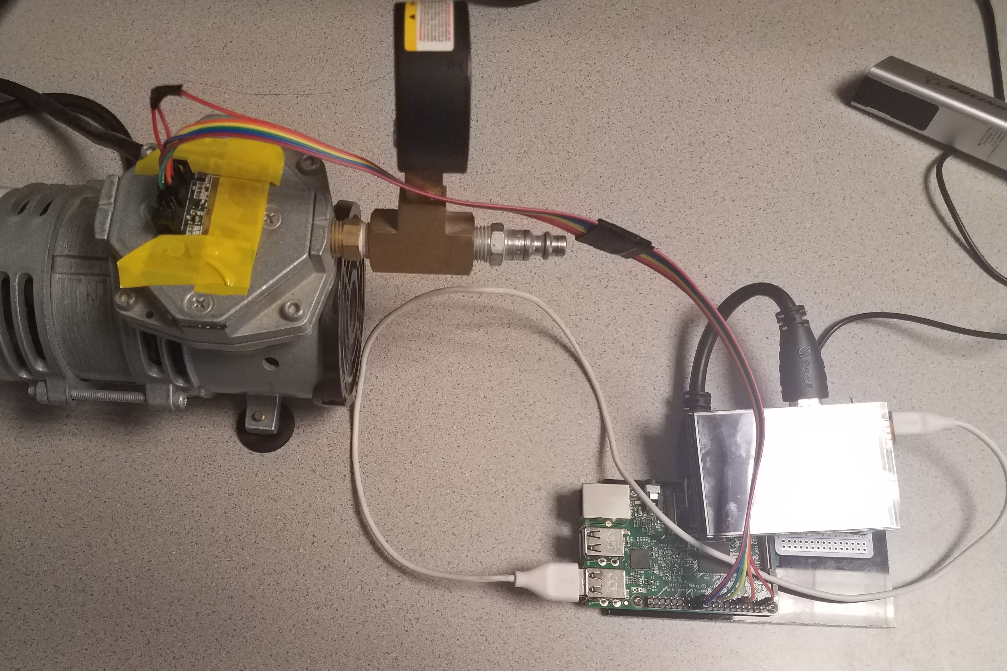
Integrated System Testing Setup

The final product was demoed on May 17 2017, a video of the demo can be seen below. The system was able to properly characterize the vibrations of a small air compressor and output the corresponding FFT plot. Although there was a slight lag in the plotting the data shown fit the expected values showing a consistent spectrum ranging from ~20 Hz to ~60hz, as to be expected of a motor running at a couple thousand RPM.

As a result of the design and implementation process we were ultimately able to design a vibration data collection system that could communicate with a peripheral accelerometer using SPI, collect and pipe data between two simultaneous programs sequestered to different cores, and provide a graphical representation of the data while processing and collecting.

The majority of design goals were met by the final implementation of the system. By combining the use of SPI, piping data between a collection and processing program, and running those programs on seperate cores we were able to create a measurement tool that was able to accurately collect and process data at high speeds. Ultimately it would indeed be possible to use this product as a tool to characterize the vibrations of a machine and assess whether there was anything abnormal.

Although the system does not currently miss any data points, the visual representation of data is slow. Additionally, the python script that processes the data runs significantly slower thatn the C code that collects the data and as a result the fifo used to pipe the data grows very quickly. It is unclear how long it would take for the fifo to get large enough to affect the Pi's performance, but it would still be a good idea to improve the speed of processing and plotting data. One possible solution for this would be to transfer the FFT process into a faster C script and pipe the resulting arrays into a python script that simply plots. doing so could help improve the overall speed and responsiveness of the system.

The current mounting platform gets the job done but there is obvious room for improvement. Screen mounting is currently unstable and there is no room for on an onboard power supply. To make the tool truly portable we would like to create a more robust enclosure, longer wires to the accelerometer, and an enclosure for the accelerometer that could provide more convenenient and secure mounting to machines rather than just tape.