BioNB 442: Lab 1

Connecting a computer to an experiment

Introduction.

This assignment will attempt to motivate the main points of this course which are:

• Converting physical quantities (such as voltages) into numbers on a computer.
• Displaying the numerical equivalents of physical qunatities in an understandable form.
• Finding patterns in very large sets of data which result from measurements.
• Converting numerical systems on the computer back into physical quantities.

Later in the semester we will be concerned with the electronic nature of the physical systems from which we are taking measurements, but for right now we will treat the electronics as a given.

Log on as user BIONB442. Make yourself a folder entitled with your netid in the My documents folder. Put all files which you may generate or download into the folder you make. You will share the account with the other students in 442.

A copy of gPRIME should be in the BIONB442 folder on your desktop. Start Matlab, open the editor, then open gPRIME with the Matlab editor and run it. Set the Device to winsound, SoundMax HD Audio, which is the computer's sound card. Add two channels.

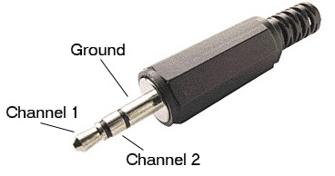
When using an audio cable as input or output, there are three connections on the plug. Normally these would be called left, right and ground, but we will call them channel 1, channel 2 and ground. A typical plug is shown below. An input to the computer goes into the line input socket, usually denoted by a blue socket. An output from the computer plugs into the earphone socket. On the machines in the lab, the two audio sockets on the front of the machine should be connected with a stereo audio cable.

Assignment

1. CD music.
   Insert a music CD into the drive. Connect the audio earphone output to the audio line-in input. Play the CD using windows media player. When you start gPRIME, choose winsound, SoundMax HD Audio as the input device, then define two channels. You should see voltage waveforms corresponding to the music output on the display.
1. As you adjust level on the Windows audio input control panel, you may be able to see the waveform clip at higher levels.
2. In gPRIME, in the view menu, turn on spectrogram visualization. Can you relate the frequency-time pattern to the music?
2. Signal generator (daqfcngen).
   Start the daqfcngen program by typing it's name at the matlab command line. A small window will appear. Typing help daqfcngen will yield an explanation of the program. It can generate one of several waveforms. Set the device to winsound0.
1. Set the function generator to produce a square wave. Feed the square wave out of the audio (earphone) port and back into the audio (line-in) port. With gPRIME running you should be able to see the square wave on the display.
2. In the view menu, turn on FFT visualization. You should see several peaks corresponding to the Fourier spectrum of the input signal. Set the frequency to 500 Hz, then 200 Hz and compare the spectrum of a square wave to a sine wave and a sawtooth. If you change the full span time of the dsiplay, you will see that the frequency estimate on the FFT display gets more accurate. Why?
3. Set the function generator to square wave and vary the duty cycle. What happens to the spectrum as the duty cycle decreases?
3. Toy retinal model.
   Connect the retinal model to the sound input of the PC. Data will be on channel 1.
1. Slide a beam of light, or a dark edge, along the 4-receptor array. You should hear a burst of simulated APs and see them on the gPRIME display plotted as voltage versus time. You may need to change the channel 1 volts/division to see the spikes.
2. Pick one of the two center LEDs and blink a light directly over it. Hold the light on for several seconds. Describe what happens. Note the amplitudes of the spikes with the light on, and after the light goes off. Each receptor has a different amplitude spike output. Which receptors are firing when the light turns on and off? There seems to be adaptation to light level. What is the time for a receptor to adapt? This question is repeated in item 5 below, more quantitatively.
3. Click the Data Analysis Mode button in gPRIME to open a separate window for detailed analysis. In the analysis window, you will need to choose a scope channel as input then use the zoom button, followed by a click and drag across a chunk of the waveform to set the vertical size. In the bottom panel set the y-axis to Energy Density (amplitude) and the x-axis to Event time. Repeat the light flashing in item 2 above. You should be able to clearly see different size spikes. Does the spike pattern suggest lateral inhibition?
4. How could you construct a definitive test for lateral inhibition? Do the experiment and report spike rates under different conditions.
5. Now set the y-axis to rate and repeat the light flashing. You should be able to quantify the rate of decrease of spike frequency after the light is either turned on or off. By clicking the log button, you should see that the decrease of spike frequency is approximately exponential. What is the 1/2 time of rate decay (You may need to turn off the auto scale and set the scale)?

Your written lab report should include:

1. Answers to all questions in the sections above.